Quick optics 101

Here's a quick fun thing to do with a telescope on a rainy day.

Try this:
- point your telescope at something bright
- remove the eyepiece and place a piece of cardboard where it should be. Move the cardboard back and forth and you'll resolve an image!

Scroll over to 30 seconds or so to see the end result.

How does it work? We know from simple optics that if you have an image a distance d0 away, that another object will appear d1 away:

where f is the focal length of your telescope. Here is a schematic of the setup. The object is labeled "O" and the image "I".

Analyzing my setup, we see that d0 = 2.5m, and f is 700mm. This means with some algebra that we should expect an image at d1 = 1.03 m.

The object is at S1 and the image at S2+S3

What happens with images from the sky?

Images from the sky are actually located so far away that d0 is very large, and as a consequence 1/d0 goes away. This means then that:
1/d1 = 1/f

So if you did the same thing with the moon, you could use it to find the focal length of your mirror!

Weather Data - Part II : The reader

So how do we extract cloud data? One method is simply by observation. However, why observe when we have the satellites to help us.

The data

The data can be found here although I currently see that the server is down (hopefully this will change soon). 

The data format

The data format is sort of summarized in this document here.

The reader

The reader written in C can be found here. However, beware, this code only works for a big endian machine. For little endian, make this substitution:
data.Preptr->npix becomes ntohl(data.Preptr->npix)


The reader (Python version)

At a recent hackathon in Montreal, I took the liberty to rewrite the library in python just to help with the visibility of this data, and also well, learn python.
Here is the source.

I would like to point out that there is also a java version written by Andre Mas here. We wrote the library in parallel just to challenge ourselves and better understand this data at a lower level.

Anyway, so what's the result?
Here is a quick result on the infrared radiance.

data set: ISCCP.DX.0.GOE-7.1991.01.01.0000 the infrared radiance measured.

Why did I choose the radiance? Because infrared is visible during the day or night. (For those who are not familiar with infrared, click this wiki link. It is like light, but longer wavelength and radiation we can't see with our eyes. But your camera can see it.) Anyway, so the satellite data also does contain data showing what the sky would look like with our eyes (visible spectrum), but then I would be limited to data that was taken during the local daytime of each place measured.


So now we have a database that can tell us the cloudiness of a certain region. Will be be able to do anything more with this? We'll see

Weather Data - Part I

(This will be a very transparent post but will be useful for the next post involved in extracting this mentioned number of prob of success)

As amateur astronomers, we all share the problem of unwanted "nebulosities" in the sky, yes I'm talking about clouds. Well, actually, if you live in a truly light pollution-free environment, then maybe it's an unwanted bok globule.

Even worse, if you want to introduce and share your passion with others, you will find these others quickly dissuaded by your failed attempts to show them the night sky because a combination of these unwanted objects and Murphy's law.

This is where statistics comes in. First let's introduce the problem and see how it is related to a simple probability distribution.

Binomial Distribution
Let's say you have observed over a few years that in the month of January, it is cloudy 2/3rds of the time. If you organize an astronomical event, you have a 1/3rd (33%) chance of success. 

Rain Date
That's difficult because most likely you'll fail. How do you improve the odds? Let's say you choose a rain date. Your chance of success is now:
(chance of success 1st day)  + (chance of failure first day) *(chance of success second day) = 1/3 + 2/3*1/3=55%

You have almost doubled your chance but not quite. What about a 2nd rain date?
Chance success = 1/3 + 2/3*1/2 + 2/3^2 *1/3 = 70%. Your chances are increasing in diminishing returns.


The importance here is that by doubling your dates, you haven't doubled your chances. It's obvious, but we need to formalize it for the next step.

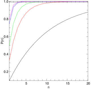
Probability of success for n-1 rain dates where perecentage success for one day is 10% (black), 33% (red), 50%(green), 75%(blue) and 80%(magenta). The horizontal black line is 99% chance of success.

So let's calculate this for multiple rain dates. The calculation is done here for n-1 rain dates above for probability of success 1/3 (red curve). The flat black line at the top of the curve is the chance of 99% success. We see that for region with 33% chance of no cloudiness, we would have to schedule 9 rain dates (total of 10 days) to beat Murphy's law with a chance of success! You see that even with 50% success you need 6 rain dates to achieve this confidence! And you can forget about it if your chance of clear skies is 10%.

What does this all mean? Basically, if you're an amateur astronomy club in a region where the chance of clear skies is 50% or lower, you'll have to think a little carefully before planning an event.

side note

I would like to note that this is an extreme simplification of the problem and that two things are important: 

1. The cloudiness on dates chosen are independent of one another. If they're dependent, this just worsens your chances. 

2. This prob of success p will probably vary month to month. The easiest simplification to this is assume the change is not large and base your calculations on the worst of the chances.

The solution

Basically, the solution to this problem (a depressing one) as an astronomy club organizer is to make sure to hold at least the number of events throughout the year that would guarantee you one event with a 99% chance of success... Holding 10 rain dates (in Montreal, where we believed the success prob to be at worst 33% for any given month) isn't really popular for any club. It's best just to hold 10 separate events throughout the year.

If you're doing this for your friends, well at least now you have a chance of warning them what they're getting into.

I'll look next at how to estimate this value of the chance of success, which I'll just call P₁.

Feel free to look at code below just to see how easy Yorick is (nice alternative to matlab). However, the user base is quite small so I would recommend using python if you're just starting. (I use Python for long code I share with others, yorick when I want to quickly program something.)

Yorick code (using source code formatter): 

1:  func binom(p,n){  
2:      /* DOCUMENT Compute the binomial prob for each  
3:      *    element n with prob p  
4:      */  
5:      res=array(0., numberof(n));  
6:      for(j = 1; j <= numberof(n); j++){  
7:          for(i = 1; i<=n(j);i++){  
8:              res(j) += p*(1-p)^(i-1);  
9:          }  
10:      }  
11:      return res;  
12:  }  
13:  n = indgen(20);  
14:  window,0;fma;  
15:  plg,binom(.10,n);  
16:  plg,binom(.33,n),color="red";  
17:  plg,binom(.5,n),color="green";  
18:  plg,binom(.75,n),color="blue";  
19:  plg,binom(.8,n),color="magenta";  
20:  pldj,n(1),.99,n(0),.99;  
21:  lbl,,"n","P(n)";  

M82 - Image Stacking

Now that I have a successful reading routine to read the images, I can process them. I have written some home image stacking routines to show how relatively simply this can be done to an amateur.

This post will be long. If you want to see the end result, just scroll to the bottom.
Please click the images to see the actual photo in full quality.

The problem
Astronomers are always starved for light. We want to capture as much light (signal) as possible to help reduce the noise. It turns out the first easy solution to capturing as much light as possible is just to leave the camera exposed to the image for hours on end. However, this does not work for two reasons:

1. Tracking systems are imperfect and the image will have shifted during the course of the measurement. This will end up with the well known star trail like effects. I will explain this soon.
2. Your detector actually saturates at a maximum value. You can think of each pixel in your camera as a mini detector. Now imagine as a bucket for light. It can only capture so many photons of light until the bucket starts to overflow. After this point it makes no sense to fill your bucket further because you won't be able to count the extra photons you've caught.

Now let's visit each of these caveats before we move on to the solution.

Tracking systems aren't perfect
The first thing all amateur astronomers learn is that, tracking systems aren't perfect. If you want to have pristine tracking, it takes a lot of work (even with the more modern GOTO mounts). Time and resources are not a leisure for hobbyists and this is a known problem.
Take a look at M82 here. The second image was taken about 1-2 min after the first. I tried my best in perfecting the tracking and I used a Celestron C8 AVX which is an equitorial GOTO mount. Still no luck, there's always a shift... You can see them below.

M82 - one image

M82 - another image. The shift relative to the previous image is marked by the arrow.

So we see there is a shift and we'd like to correct for it. It turns out this shift is not that big, approx 1/5th of a pixel per second. Thus if I expose the camera for 10 seconds, the image will have moved at most 2 pixels or so. This can actually be corrected for quite easily. Before explaining the correction, let's discuss the second problem: that of image saturation.

Image Saturation
A good example of image saturation (that isn't a star) is one our our planets: Saturn. The planets are some of the brightest objects in the sky. No wonder the word comes from the greek word astēr planētēs which means "wandering star". They're one of the brightest "stars" in the sky but oh... such rebels!

So what happens if I overexpose the image? See for yourself (units are arbitrary):
 

Overexposed Saturn Image

A cross section of the overexposed image.

 Take a look at the image. Near the center of the object, all the values look to have the same color. Even worse, by looking at a cross section, you see that they are the same! This is the result of overexposure. The little "buckets" of light in your camera can only gather so much energy before it spills over. Each little bucket here could only hold so much before it could not report any more signal. So how do you correct for this issue? Easy, you read out multiple images before these buckets "spill over," as will be described next.

How do you correct for this?
Now how would one go about correcting for this? The correction is actually a two-piece process:

1. Take multiple images of shorter exposure before the light buckets spill over, and before the image shifts appreciably.
2. Re-shift the images back in position and then average them.

The first piece is simple. I have taken here 10 second exposures. This is enough to avoid both saturation and star trails. The second piece is explained in two steps:
1. The shifting process
2. The averaging process

First Step: The image shifting process
One method is simple, you can manually shift each image so that it looks like it overlays on top of the image. But how do you know when you've shifted by just the right amount? Easy: Just take the absolute value of the difference of the two images. Here is a result of the absolute value of the difference of two M82 images shown earlier and look at just one star:

M82 difference of two images, zoom in on a star.

The shift is now pretty clear. It looks to be 5 pixels in x and 23 pixels in y. Now, let's shift these images by this amount and take the difference again:

Difference of two images of M82, where the second is shifted by 5 pixels in x and 23 pixels in y.

We can see the image now looks almost to be zero (although not perfect). Now, a sensible solution would be to have a program try to take the absolute value of the difference of images for a few values, and check to see where there is a minimum. Where you find your minimum will be the region that the image has most likely shifted. A sensible solution.

It turns out there is a slightly better and quicker trick using fourier transforms, but I have run out of time. I will post it later with code and examples. Anyway, so for now we have some way of determining the shift of the images numerically.


Second step: average them!
So now, you have a sequence of images, and you also have a method of shifting them back in place. In other words, you have a sequence of the same image. So what next?
Images will always contain noise, like it or not, which will amount to graininess in your images. There is an easy way to reduce this graininess. It is well known in statistics that to reduce the noise in any measurement, all you need to do is make the same measurement again and again and average the results together. Say you averaged 10 measurements together. If each measurement was truly independent, then your noise (graininess) will be reduced by a factor of 1/sqrt(10) where "sqrt" means "the square root of".  If you have N images, then your noise is reduced by 1/sqrt(N). Remember, this only holds for independent measurements.

Here is an example. I take a cross section of M82 and I plot it below. I then take the average of 20 independent measurements of M82 and plot the cross section in red. The graininess (noise) appears to have been reduced by 1/sqrt(20) or approximately 1/5th. So it works!

 

The Final Result
So there you have it. Now let's see what happens when we apply this to M82 as below:

M82 - One image 800ISO 10 s exposure with Nikon D90, converted to grayscale, byte-scaled between 60 and 100 ADU. Click to see the actual photo!

 And shift+stack it:

M82 - Stacked images at 800ISO 10 s exposure with Nikon D90, converted to grayscale, byte-scaled between 60 and 100 ADU. Click to see the actual photo!

Voila! A much nicer image. Note that this has been done with only 20 images, in grayscale and an extremely light polluted (McGill Observatory) area. It would be interesting to compare the same measurements (on the same day, with same moon phase) both at the heart of light polluted montreal and its darker rural skies.

Astrophotography Part 4 - The Color Matrix

Log Entry
The Color Matrix

This will be the last piece in a series of entries dedicated to unencoding the Nikon Images. I mentioned in the previous post how to huffman decode the image. It turns out, that each value decoded for each pixel is still not the final value for each pixel in the image. Before I mention the extra piece missing, let's go into how digital cameras record color.

The Nikon D90 is a color camera. This means that it registers not only brightness information, but color as well. We learn in kindergarten that most of all colors we see can be made up of a linear combination of three primary colors: red, green and blue. So the simple way to obtain a color image is to have a set of three images containing the intensity for each the red, green and blue colors. 

So how do you take a red, green and blue image? A simple solution is simply to take three separate images. Before taking each, place a red filter, then a green filter, then a blue filter.

It turns out that this simple picture in CCD cameras is not that practical. How do you insert the filter? How do you switch it fast enough so that you can take three images for the price of one?

Bryce Bayer, while working for Eastman Kodak, found a solution for colour digital cameras. First, let’s discuss the way digital cameras work. Digital cameras measure an image focused on a chip with mini detectors we call pixels. Each pixel basically registers the intensity of the light impinging on it with some units we usually arbitrarily label as Analog to Digital Units (ADU).

The idea Bayer introduced is to have each pixel dedicated to measuring only one of the three primary colors, with twice as many measuring green as opposed to red and blue to mimic the human eye. This was simple to implement as all that was necessary was to permanently place a filter on each pixel. One could then use simple interpolation techniques to then recover the colour information for the rest of the pixels. He may have passed away 1.5 years ago, but his legacy is in 99% of cameras today.

Here is a sample Bayer Matrix of what I believe the Nikon images contain (after some playing around):

Sample Bayer Matrix from the Nikon D90.

In this matrix, you see one 2x2 matrix repeated throughout the whole CCD chip.

Back to the RAW Image
The reason why I am discussing the color matrix here is that it turns out, when reading the RAW image from the Nikon D90, each value obtained is actually the difference to add in for a previous value. Here goes, this will be a little complicated. I will try to point out the key points but you may need to do a little bit of work to get this on your own (basically, I don't have much time):

Read the first huffman byte sequence based on the tree in a previous post. Next, read that number of bits as your value. When you obtain the value, follow the following rule. If:
1. The leading bit of this value is zero: Subtract 2^len from it (where len is the length of the bitstream)
2. The leading bit is not zero: keep it as is.

Next, this value needs to be summed to the previous value. The previous value is defined by the following rule:
1. If the current pixel is within the first two rows and the first two columns: (first Bayer matrix element) The previous value is defined as the value from the vpred matrix obtained with the linearization curve. This matrix is a 2x2 matrix and is obtained with the linearization curve. A summary will be written eventually (not yet, when I have time). You may find information on vpred here for now.
2. If the current pixel is not within the first two rows but within the first two columns: The previous value is defined as the previous element in the Bayer matrix (that is the previous element two rows above here).
3. If the current pixel is not within the first row or the first column: The previous value is defined as the previous element in the Bayer matrix horizontally to the left (so two columns back)

There you go. Now all you need to do is for each pixel, follow the leading bit rule and sum the previous value to it which is defined by the rules above.

If you think about it, this makes sense. One would always expect a pixel close by not to differ by much, so you save space by saving pixel differences as opposed to pixel values. Note with these rules, you are always forced to add the difference to a pixel not more than 2 pixels away. The underlying logic is much simpler than the explanation.

Here is a slightly edited version of dcraw's code to point out what needs to be done:
 
for(row = 0; row < imgheight; row++){
     for (col=0; col < imgwidth; col++) {
      len = gethuff(huff);//read the next huff from byte sequence
      diff = (getbits(len));//get the next len bits
      if ((diff & (1 << (len-1))) == 0)
        diff -= (1 << len); //subtract 2^len if leading bit zero
      if (col < 2)  //if in the first two columns
           hpred[col] = (vpred[row & 1][col] += diff);
      else         hpred[col & 1] += diff;//else      
 //RAW is index into raw image, curve is the interpolation from 
//the value based on the linearization curve. you can ignore the 
//latter step and always do the interpolation later.
RAW(row,col) = curve[LIM((short)hpred[col & 1],0,0x3fff)];
    }
}

And that's it. To avoid any copyright issues, I must cite Dave Coffin and link to his full source code here.  (Click dcraw link in page)
          

One more small detail...
It turns out that the images you will read will be 4352 x 2868 pixels (the dimensions are also specified in the EXIF tags). The columns from 4311 to 4352 actually just contain garbage (or they look like garbage to me, very high values). I just ignore them and use a 4310 x 2868 sub image. Note that this is still larger than the maximum resolution of the Nikon D90 (4,288 × 2,848 pixels from wikipedia), but who cares, it looks like good data. It is probably good to keep this in mind though.

Interpolating from Bayer to RGB
A simple way to interpolate the image is convert each 2x2 element to an RGB pixel and I will do this for all my pictures here.
The dimensions of the Nikon raw images are 4352 x 2868. So for these images, my final resolution will be 2176 x 1434 pixels. This is fine enough for me.

Here is some quick pseudo code to obtain each color from an image:
img = read_image();
RED = img(1::2,1::2);
GREEN = (img(2::2,1::2) + img(1::2,2::2))*.5;
BLUE = img(2::2,2::2);

Now let's see if it worked and just plot the gray image by calculating:
GRAY = RED + GREEN + BLUE;

where min:max:skip is a notation meaning starting from index min up to max, skipping skip values every time. When left blank, min defaults to the beginning, max to the end and skip to 1 (so don't skip). 

Let's try this with a moon image I took:

The moon at 800 ISO 1/4000 s exposure with the Nikon D90.

And voila.

This concludes the image reading portion of the Nikon images. Any questions, feel free to comment. If you are interested in source code, please comment. I can include Dave Coffin's code with a diff file showing how to make it just a raw image reader.

I will try to write up a reference sort of like here but a little more complete so the next person will not feel as frustrated as I did. Good luck!

Nikon D90 - Dark Analysis

Before I begin, I will introduce a piece of notation.
Log Entry ####: - Specifies a log entry
Summary Entry #####: - Specifies a summary

This blog is mostly a logbook but every once in a while I will try to summarize a few interesting things discovered along the way that may be beneficial to others. The following entry is a log entry.

Nikon D90 Dark Analysis
Log Entry Friday July 4th, 2014 8:14pm  


I have ended up interfacing Dave Coffin's dcraw C code into yorick. It took a bit of time to figure out which pieces were essential and which not. I will not post it here just to avoid any copyright issues, but I'll post a summary of the steps later. It is open source but he does request the full source code to be available. If you would like to see it, please comment here or contact me and I will reply.

What I can say is that his code is wonderful and efficient (although obfuscated). If starting to read any raw image, I recommend using his code and interfacing it into your matlab or yorick environment as a starting point. The main piece you need is the call to "load_raw", just look for that in the main function.

Before plotting any images, I first look at the dark images. In this example, I turn the RAW image into a black and white image. Basically, I take the RGB information and just sum them. Here they are:

400 ISO dark near 0 degrees Celsius for a 10 second exposure. This is an average of 6 darks. The inset is the plot of the intensity along the red line (in ADU).

800 ISO dark near 0 degrees Celsius, for a 10 second exposure. This is an average of 5 darks. The inset is the plot of the intensity along the red line (in ADU).

What I would like to point out is how nice these dark images are. The average ADU levels are very close to zero (the dynamic range of the RAW images is 0 to 4096 ADU per pixel). Keep in mind this is a 10 second exposure as well. From now on, I will ignore the dark images since it turns out that the images themselves will have a much higher signal.

M82

This one will be quick and easy. I have given up on extracting the images manually, not because it's hard, but because the interpreted programming language I'm using has a lot of overhead and I will need to re-write everything in C and have yorick interface it as a plugin. (Each image takes about 3-4min to decode...) The following is done simply using the dcraw code + image magick + gimp:

M82 - The cigar galaxy. Nikon D90 800 ISO.

Here is an image of M82, the cigar galaxy. This image was obtained by stacking together 13 images. It was taken in downtown Montreal. The light pollution is so large in Montreal that the contrast between the features of the galaxy and the sky is very low.

More analysis on this later.

All processing was done with Gimp, an open-source photoshop alternative. The procedure is called image stacking. Image stacking means just computing an average image of a set of images to increase the signal to noise. However, with amateur astronomy photos, there is one extra detail. As the evening progresses, your tracking system may not be perfect and you will find that your images may shift a little. By using gimp and its difference feature, it is possible to correct for this shift before you obtain the average (note this is much trickier for rotations so be careful not to rotate your camera between photos, and use an EQ mount to avoid field rotation). You'll probably want to worry about dark images and flatfield corrections as well but these are details to the process that become obvious once you do it.

One small interesting feature. A supernova occurred in this particular galaxy and the light curve from the AAVSO  shows that it is probably around 15 magnitude (picture taken near May 7th, 2014).

AAVSO data. Black curve is the visible data.

It turns out this means that it is 10 times weaker than a 12.5 magnitude star (10 times brightness every 2.5 magnitude). Universe today has a nice picture showing a 12.2 magnitude star around the area. I'll elucidate it here:

M82 with its supernova and some surrounding stars.

And there you have it. M82 in all its glory with its supernova SN 2014J, surrounded by an obnoxious light pollution background.