M82 - Image Stacking

Now that I have a successful reading routine to read the images, I can process them. I have written some home image stacking routines to show how relatively simply this can be done to an amateur.

This post will be long. If you want to see the end result, just scroll to the bottom.
Please click the images to see the actual photo in full quality.

The problem
Astronomers are always starved for light. We want to capture as much light (signal) as possible to help reduce the noise. It turns out the first easy solution to capturing as much light as possible is just to leave the camera exposed to the image for hours on end. However, this does not work for two reasons:

1. Tracking systems are imperfect and the image will have shifted during the course of the measurement. This will end up with the well known star trail like effects. I will explain this soon.
2. Your detector actually saturates at a maximum value. You can think of each pixel in your camera as a mini detector. Now imagine as a bucket for light. It can only capture so many photons of light until the bucket starts to overflow. After this point it makes no sense to fill your bucket further because you won't be able to count the extra photons you've caught.

Now let's visit each of these caveats before we move on to the solution.

Tracking systems aren't perfect
The first thing all amateur astronomers learn is that, tracking systems aren't perfect. If you want to have pristine tracking, it takes a lot of work (even with the more modern GOTO mounts). Time and resources are not a leisure for hobbyists and this is a known problem.
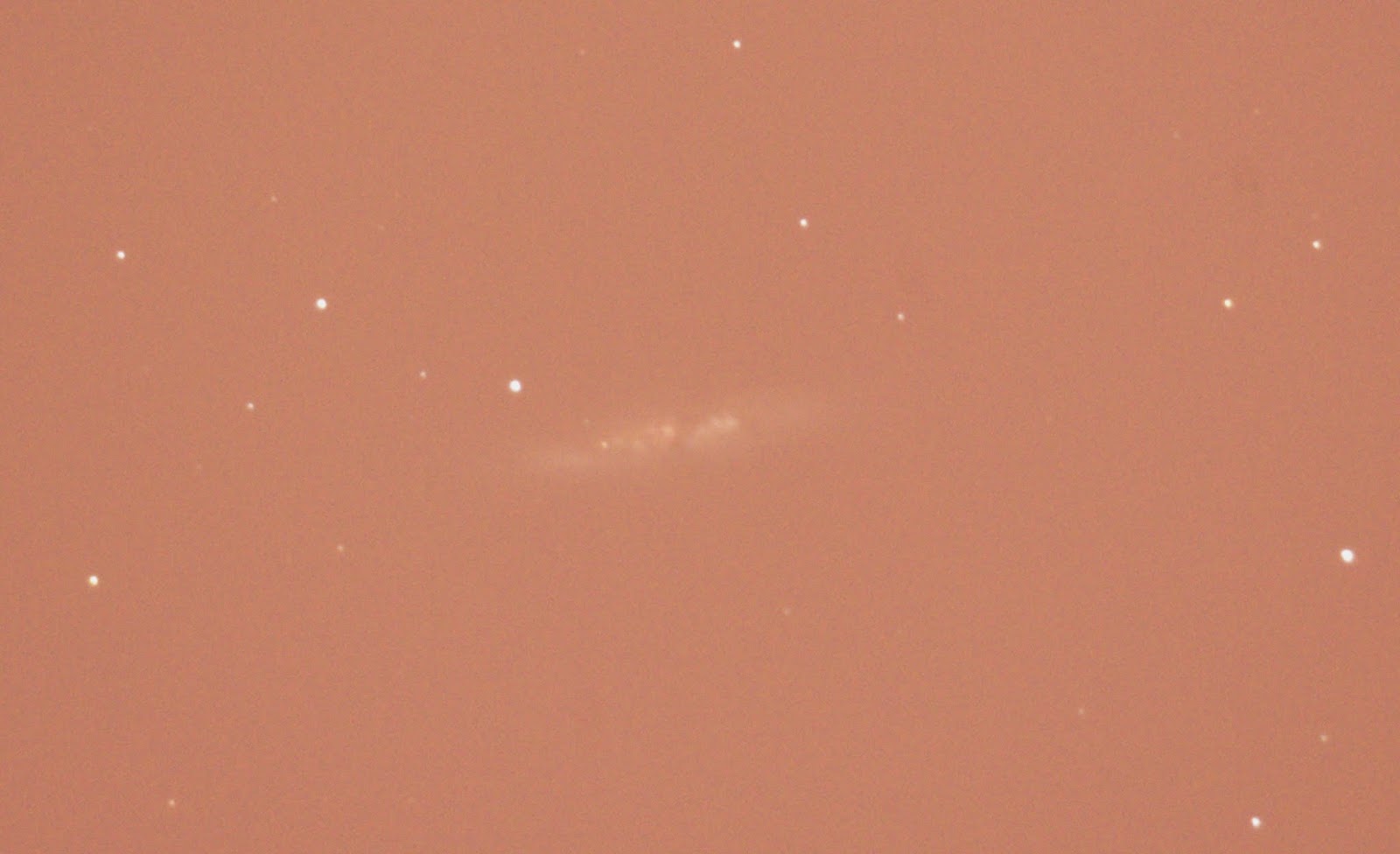
Take a look at M82 here. The second image was taken about 1-2 min after the first. I tried my best in perfecting the tracking and I used a Celestron C8 AVX which is an equitorial GOTO mount. Still no luck, there's always a shift... You can see them below.

M82 - one image

M82 - another image. The shift relative to the previous image is marked by the arrow.

So we see there is a shift and we'd like to correct for it. It turns out this shift is not that big, approx 1/5th of a pixel per second. Thus if I expose the camera for 10 seconds, the image will have moved at most 2 pixels or so. This can actually be corrected for quite easily. Before explaining the correction, let's discuss the second problem: that of image saturation.

Image Saturation
A good example of image saturation (that isn't a star) is one our our planets: Saturn. The planets are some of the brightest objects in the sky. No wonder the word comes from the greek word astēr planētēs which means "wandering star". They're one of the brightest "stars" in the sky but oh... such rebels!

So what happens if I overexpose the image? See for yourself (units are arbitrary):
 

Overexposed Saturn Image

A cross section of the overexposed image.

 Take a look at the image. Near the center of the object, all the values look to have the same color. Even worse, by looking at a cross section, you see that they are the same! This is the result of overexposure. The little "buckets" of light in your camera can only gather so much energy before it spills over. Each little bucket here could only hold so much before it could not report any more signal. So how do you correct for this issue? Easy, you read out multiple images before these buckets "spill over," as will be described next.

How do you correct for this?
Now how would one go about correcting for this? The correction is actually a two-piece process:

1. Take multiple images of shorter exposure before the light buckets spill over, and before the image shifts appreciably.
2. Re-shift the images back in position and then average them.

The first piece is simple. I have taken here 10 second exposures. This is enough to avoid both saturation and star trails. The second piece is explained in two steps:
1. The shifting process
2. The averaging process

First Step: The image shifting process
One method is simple, you can manually shift each image so that it looks like it overlays on top of the image. But how do you know when you've shifted by just the right amount? Easy: Just take the absolute value of the difference of the two images. Here is a result of the absolute value of the difference of two M82 images shown earlier and look at just one star:

M82 difference of two images, zoom in on a star.

The shift is now pretty clear. It looks to be 5 pixels in x and 23 pixels in y. Now, let's shift these images by this amount and take the difference again:

Difference of two images of M82, where the second is shifted by 5 pixels in x and 23 pixels in y.

We can see the image now looks almost to be zero (although not perfect). Now, a sensible solution would be to have a program try to take the absolute value of the difference of images for a few values, and check to see where there is a minimum. Where you find your minimum will be the region that the image has most likely shifted. A sensible solution.

It turns out there is a slightly better and quicker trick using fourier transforms, but I have run out of time. I will post it later with code and examples. Anyway, so for now we have some way of determining the shift of the images numerically.


Second step: average them!
So now, you have a sequence of images, and you also have a method of shifting them back in place. In other words, you have a sequence of the same image. So what next?
Images will always contain noise, like it or not, which will amount to graininess in your images. There is an easy way to reduce this graininess. It is well known in statistics that to reduce the noise in any measurement, all you need to do is make the same measurement again and again and average the results together. Say you averaged 10 measurements together. If each measurement was truly independent, then your noise (graininess) will be reduced by a factor of 1/sqrt(10) where "sqrt" means "the square root of".  If you have N images, then your noise is reduced by 1/sqrt(N). Remember, this only holds for independent measurements.

Here is an example. I take a cross section of M82 and I plot it below. I then take the average of 20 independent measurements of M82 and plot the cross section in red. The graininess (noise) appears to have been reduced by 1/sqrt(20) or approximately 1/5th. So it works!

 

The Final Result
So there you have it. Now let's see what happens when we apply this to M82 as below:

M82 - One image 800ISO 10 s exposure with Nikon D90, converted to grayscale, byte-scaled between 60 and 100 ADU. Click to see the actual photo!

 And shift+stack it:

M82 - Stacked images at 800ISO 10 s exposure with Nikon D90, converted to grayscale, byte-scaled between 60 and 100 ADU. Click to see the actual photo!

Voila! A much nicer image. Note that this has been done with only 20 images, in grayscale and an extremely light polluted (McGill Observatory) area. It would be interesting to compare the same measurements (on the same day, with same moon phase) both at the heart of light polluted montreal and its darker rural skies.

Astrophotography Part 4 - The Color Matrix

Log Entry
The Color Matrix

This will be the last piece in a series of entries dedicated to unencoding the Nikon Images. I mentioned in the previous post how to huffman decode the image. It turns out, that each value decoded for each pixel is still not the final value for each pixel in the image. Before I mention the extra piece missing, let's go into how digital cameras record color.

The Nikon D90 is a color camera. This means that it registers not only brightness information, but color as well. We learn in kindergarten that most of all colors we see can be made up of a linear combination of three primary colors: red, green and blue. So the simple way to obtain a color image is to have a set of three images containing the intensity for each the red, green and blue colors. 

So how do you take a red, green and blue image? A simple solution is simply to take three separate images. Before taking each, place a red filter, then a green filter, then a blue filter.

It turns out that this simple picture in CCD cameras is not that practical. How do you insert the filter? How do you switch it fast enough so that you can take three images for the price of one?

Bryce Bayer, while working for Eastman Kodak, found a solution for colour digital cameras. First, let’s discuss the way digital cameras work. Digital cameras measure an image focused on a chip with mini detectors we call pixels. Each pixel basically registers the intensity of the light impinging on it with some units we usually arbitrarily label as Analog to Digital Units (ADU).

The idea Bayer introduced is to have each pixel dedicated to measuring only one of the three primary colors, with twice as many measuring green as opposed to red and blue to mimic the human eye. This was simple to implement as all that was necessary was to permanently place a filter on each pixel. One could then use simple interpolation techniques to then recover the colour information for the rest of the pixels. He may have passed away 1.5 years ago, but his legacy is in 99% of cameras today.

Here is a sample Bayer Matrix of what I believe the Nikon images contain (after some playing around):

Sample Bayer Matrix from the Nikon D90.

In this matrix, you see one 2x2 matrix repeated throughout the whole CCD chip.

Back to the RAW Image
The reason why I am discussing the color matrix here is that it turns out, when reading the RAW image from the Nikon D90, each value obtained is actually the difference to add in for a previous value. Here goes, this will be a little complicated. I will try to point out the key points but you may need to do a little bit of work to get this on your own (basically, I don't have much time):

Read the first huffman byte sequence based on the tree in a previous post. Next, read that number of bits as your value. When you obtain the value, follow the following rule. If:
1. The leading bit of this value is zero: Subtract 2^len from it (where len is the length of the bitstream)
2. The leading bit is not zero: keep it as is.

Next, this value needs to be summed to the previous value. The previous value is defined by the following rule:
1. If the current pixel is within the first two rows and the first two columns: (first Bayer matrix element) The previous value is defined as the value from the vpred matrix obtained with the linearization curve. This matrix is a 2x2 matrix and is obtained with the linearization curve. A summary will be written eventually (not yet, when I have time). You may find information on vpred here for now.
2. If the current pixel is not within the first two rows but within the first two columns: The previous value is defined as the previous element in the Bayer matrix (that is the previous element two rows above here).
3. If the current pixel is not within the first row or the first column: The previous value is defined as the previous element in the Bayer matrix horizontally to the left (so two columns back)

There you go. Now all you need to do is for each pixel, follow the leading bit rule and sum the previous value to it which is defined by the rules above.

If you think about it, this makes sense. One would always expect a pixel close by not to differ by much, so you save space by saving pixel differences as opposed to pixel values. Note with these rules, you are always forced to add the difference to a pixel not more than 2 pixels away. The underlying logic is much simpler than the explanation.

Here is a slightly edited version of dcraw's code to point out what needs to be done:
 
for(row = 0; row < imgheight; row++){
     for (col=0; col < imgwidth; col++) {
      len = gethuff(huff);//read the next huff from byte sequence
      diff = (getbits(len));//get the next len bits
      if ((diff & (1 << (len-1))) == 0)
        diff -= (1 << len); //subtract 2^len if leading bit zero
      if (col < 2)  //if in the first two columns
           hpred[col] = (vpred[row & 1][col] += diff);
      else         hpred[col & 1] += diff;//else      
 //RAW is index into raw image, curve is the interpolation from 
//the value based on the linearization curve. you can ignore the 
//latter step and always do the interpolation later.
RAW(row,col) = curve[LIM((short)hpred[col & 1],0,0x3fff)];
    }
}

And that's it. To avoid any copyright issues, I must cite Dave Coffin and link to his full source code here.  (Click dcraw link in page)
          

One more small detail...
It turns out that the images you will read will be 4352 x 2868 pixels (the dimensions are also specified in the EXIF tags). The columns from 4311 to 4352 actually just contain garbage (or they look like garbage to me, very high values). I just ignore them and use a 4310 x 2868 sub image. Note that this is still larger than the maximum resolution of the Nikon D90 (4,288 × 2,848 pixels from wikipedia), but who cares, it looks like good data. It is probably good to keep this in mind though.

Interpolating from Bayer to RGB
A simple way to interpolate the image is convert each 2x2 element to an RGB pixel and I will do this for all my pictures here.
The dimensions of the Nikon raw images are 4352 x 2868. So for these images, my final resolution will be 2176 x 1434 pixels. This is fine enough for me.

Here is some quick pseudo code to obtain each color from an image:
img = read_image();
RED = img(1::2,1::2);
GREEN = (img(2::2,1::2) + img(1::2,2::2))*.5;
BLUE = img(2::2,2::2);

Now let's see if it worked and just plot the gray image by calculating:
GRAY = RED + GREEN + BLUE;

where min:max:skip is a notation meaning starting from index min up to max, skipping skip values every time. When left blank, min defaults to the beginning, max to the end and skip to 1 (so don't skip). 

Let's try this with a moon image I took:

The moon at 800 ISO 1/4000 s exposure with the Nikon D90.

And voila.

This concludes the image reading portion of the Nikon images. Any questions, feel free to comment. If you are interested in source code, please comment. I can include Dave Coffin's code with a diff file showing how to make it just a raw image reader.

I will try to write up a reference sort of like here but a little more complete so the next person will not feel as frustrated as I did. Good luck!

Nikon D90 - Dark Analysis

Before I begin, I will introduce a piece of notation.
Log Entry ####: - Specifies a log entry
Summary Entry #####: - Specifies a summary

This blog is mostly a logbook but every once in a while I will try to summarize a few interesting things discovered along the way that may be beneficial to others. The following entry is a log entry.

Nikon D90 Dark Analysis
Log Entry Friday July 4th, 2014 8:14pm  


I have ended up interfacing Dave Coffin's dcraw C code into yorick. It took a bit of time to figure out which pieces were essential and which not. I will not post it here just to avoid any copyright issues, but I'll post a summary of the steps later. It is open source but he does request the full source code to be available. If you would like to see it, please comment here or contact me and I will reply.

What I can say is that his code is wonderful and efficient (although obfuscated). If starting to read any raw image, I recommend using his code and interfacing it into your matlab or yorick environment as a starting point. The main piece you need is the call to "load_raw", just look for that in the main function.

Before plotting any images, I first look at the dark images. In this example, I turn the RAW image into a black and white image. Basically, I take the RGB information and just sum them. Here they are:

400 ISO dark near 0 degrees Celsius for a 10 second exposure. This is an average of 6 darks. The inset is the plot of the intensity along the red line (in ADU).

800 ISO dark near 0 degrees Celsius, for a 10 second exposure. This is an average of 5 darks. The inset is the plot of the intensity along the red line (in ADU).

What I would like to point out is how nice these dark images are. The average ADU levels are very close to zero (the dynamic range of the RAW images is 0 to 4096 ADU per pixel). Keep in mind this is a 10 second exposure as well. From now on, I will ignore the dark images since it turns out that the images themselves will have a much higher signal.

M82

This one will be quick and easy. I have given up on extracting the images manually, not because it's hard, but because the interpreted programming language I'm using has a lot of overhead and I will need to re-write everything in C and have yorick interface it as a plugin. (Each image takes about 3-4min to decode...) The following is done simply using the dcraw code + image magick + gimp:

M82 - The cigar galaxy. Nikon D90 800 ISO.

Here is an image of M82, the cigar galaxy. This image was obtained by stacking together 13 images. It was taken in downtown Montreal. The light pollution is so large in Montreal that the contrast between the features of the galaxy and the sky is very low.

More analysis on this later.

All processing was done with Gimp, an open-source photoshop alternative. The procedure is called image stacking. Image stacking means just computing an average image of a set of images to increase the signal to noise. However, with amateur astronomy photos, there is one extra detail. As the evening progresses, your tracking system may not be perfect and you will find that your images may shift a little. By using gimp and its difference feature, it is possible to correct for this shift before you obtain the average (note this is much trickier for rotations so be careful not to rotate your camera between photos, and use an EQ mount to avoid field rotation). You'll probably want to worry about dark images and flatfield corrections as well but these are details to the process that become obvious once you do it.

One small interesting feature. A supernova occurred in this particular galaxy and the light curve from the AAVSO  shows that it is probably around 15 magnitude (picture taken near May 7th, 2014).

AAVSO data. Black curve is the visible data.

It turns out this means that it is 10 times weaker than a 12.5 magnitude star (10 times brightness every 2.5 magnitude). Universe today has a nice picture showing a 12.2 magnitude star around the area. I'll elucidate it here:

M82 with its supernova and some surrounding stars.

And there you have it. M82 in all its glory with its supernova SN 2014J, surrounded by an obnoxious light pollution background.

Quick Way to Decode a Huffman Table

(2nd version - my previous version was erased)

The scope of this blog is astronomy DIY tinkering. The current goal is to develop a set of routines to process some nice amateur astronomer photos and (hopefully) learn some neat stuff along the way. However, it is necessary to learn some techniques/tools out of the scope of the blog (or logbook) along the way sometimes, which is what makes any hobby fun. I came across a neat shortcut to decoding a Huffman table the other day and thought I would share it. It is part of Dave Coffin's dcraw code. You can find the code here. (Look for the make_decoder_ref function in the code)

Huffman Tree - Short Intro
First of all, what is a Huffman tree? I won't go into too many details because you can find it online but basically it is something like this (for the Nikon D90 images for example):
 

Huffman tree for the Nikon D90 NEF files

When reading a bit pattern, you basically start from the root of the tree, move down and left for a 0, down and right for a 1 until you reach a leaf. When you reach a leaf, that's your first data segment in your code (So 011 would yield 0x03 in this example). This variable length coding is quite good for compression where certain bit patterns occur more often than others (so you'd have the more frequent bit pattern represented by a shorter string, with the trade off that the less frequent bit pattern may be represented by a longer string).

Okay, so walking through trees are quite implemented by some sort of referencing mechanism (pointers or arrays). You just follow the arrow like in the diagram. This is usually fine since the depth of trees is logarithmic. It gets even better when the trees are not simply binary, but the behavior is the same.

But why not speed up if you can?

The trick
There is a way to access with one access as opposed to "following the arrows". The trick to getting this to work is the way the huffman table is made. Since one doesn't care about what the exact huffman code is, one can skew the tree. We can re-arrange is such that:

1. For every leaf at some depth d, the next available leaf to the right is at either the same depth d or lower.
2.  There is only one node that is not a leaf and has only one child. (Will make sense later on)

If you look at the Nikon tree above, you'll notice that it seems that they've done just that which is neat. There was no value for the righter most value so it is possible this is not implemented by Nikon.

We then have two properties:

1. From any leaf, the next leaf to the right is a bit pattern of same or greater length than the previous bit pattern
2. (general property of binary tree) At the same depth d, walking along the nodes from left to right is the same as adding 1 to the size d bit string that would represent it. You can prove this by induction. The base case would be a tree of depth 1 of which you could tack on two trees of depth onto as the n+1 case for ex:



Sample Binary tree

Knowing this, let's take the value of every leaf and just pad it to the right with zeros, so that it is as long as the longest possible bit pattern in the Huffman tree. So if my maximum length was 10 and my current bit pattern was 010111, it would then be: 0101110000 for a total length of 10.

Now, let me walk from one leaf of length d1 with pattern A1 and compare if o the next leaf to the right (which may be at a lower depth) A2 with depth d2:
A1(0...0)
A2(0...0)

I know the following. At depth d, I must walk along the nodes to the right at the same depth, so the first d bits must be (A1+1). After this, I know the rest must be zero padded. This is because there are two possible choices for the next leaf:

1. It is the same depth as the previous leaf so the rest of the values are zero padded.
2. It is deeper. This means we're on a node again. Since each node must have two children, then as we walk down the tree, we can always take the node to the left until we reach a leaf (which has 0 children of course).

Implementation
With all this information, there actually ends up being a quick way to implement the access of the huffman code. Let's say the maximum depth of the tree was D. All we need to do is make an array of size 2^D.
We fill the elements as follows:

huff = lengths = array(0., 2^D);
For each depth d:
          For each leaf from i = 1 to N
                  Fill the next 2^(D-d) elements in huff with the first code. Store the length d in a separate array for that code as well.
          end for
end for

And voila. Now, the read process is as follows:
1. Read D bits from buffer. If end of data, exit.
2. huff[D] is the next result and the length of the code was length[D]
3.  Only move cursor in buffer by D-length[D] and go back to 1

Notice that for each code one access is performed. No tree walkthrough necessary!

Drawbacks
This only works for skewed trees with the two-child rule stated earlier. Although it is easy to make a huffman tree following these rules (just loop through finding the min depth leaf and moving it right as you would for sorting), you can't do this if the code you're trying to decode has been encoded. This encoding scheme looks clearly intentional on Nikon's part and is a neat little trick.

Comments suggestions? I view this as a shared logbook. I try to share what I find neat and hope it to interest/inspire others to dig around outside their boundaries of expertise (these ideas are new to me). I hope this to be useful information to some person some day!

(astrophotos soon, and two other projects lined up, but not implemented... :-D)

Unencoding the Nikon Images - Part 3

Astrophotography Part 3 - Unencoding the Nikon D90 Images

I don't have much time other than weekends and metro rides where I can read source code on my Kindle Fire so this is going slowly...

Anyway, there is some code out there written by Dave Coffin to decode most image formats. It's wonderfully written, but it's quite terse and not commented too often. Anyway, the images for the Nikon D90 are huffman encoded, and the decoding tree is well... not in the F*$&@$G file!


Dave Coffin's code contains the decoding tree which is as follows:
 { 0,1,5,1,1,1,1,1,1,2,0,0,0,0,0,0,    /* 12-bit lossy */
      5,4,3,6,2,7,1,0,8,9,11,10,12, ?? } //ignore the "??" for now

There are two pieces to this code:

1. The occurences: The first 16 numbers are a separate quantity in themself. The nth position refers to the number of occurrences of an n-length code. 
2. The leaves : The rest of the data are the leaves. Notice that the sum of the for 16 numbers should equal the number of leaves. Also note that this describes 12 bit data and that there are 12 leaves (there seems to be a typo in Dave Coffin's code so there is a missing leaf, hence the "??").

Anyway, making the tree, you should find that the code goes as follows:

00 - 5
010 - 4
011 - 3
100 - 6
101 - 2
110 - 7
1110 - 1
11110 - 0
111110 - 8
1111110 - 9
11111110 - 11
111111110 - 10
1111111110 - 12
1111111111 - ??
I have no clue what the last value is because it seems that his source code doesn't have it. In either case, I have checked and this value never occurs in my image so we're all good. But it would be a good idea to have an error message returned it this value is ever found.

What these values mean

It turns out that this code does not give you the image itself. It actually gives you the number of bytes to read after the code for each pixel. So the decoding pattern would be (at iteration n):

1. Find the next huffman code
2. Decode it and read that number of bits. This value will be used for the nth pixel
3. repeat for n+1

Before continuing, we can make the following remark. In the huffman encoding scheme, the length of the bit pattern is more or so inversely related to the frequency. So we see the number of bits returned is usually in the ballpark of 2-7 bits, with 0,1,8 being rarer.
Also, the order in which you read the pixels is obviously important. The array dimensions should be 2868x4352. So, in this case that an nth pixel is located in position (assuming 0 based indexing. For 1-based, subtract 1 from n first then add 1 after the operation to result):
n/2868 + n%2868 4352


Anyway, that's the basic idea for now. The next step is to understand the color matrix, which I'll get to when I find time. The next image I will show will be a very bad (false color) plot of the raw pixels, so you are warned. After this maybe some discussions on code. There is a fast technique Dave Coffin uses to decode a huffman table (and took some time thinking about it on the metro while reading it) that is pretty neat. I could not find documentation on this anywhere.

False Color plot of the image so far. This one is of the moon.

A zoom on the plot. Notice the periodicity in x and y.

Astrophotography Part 2 : The Linearization Curve

Okay, so last post I was trying to understand the format of the Nikon Images. So they are standard TIFF format which contains some sort of header followed by locations to Image File Directories (IFD's) which each contain tiff tags which point to the image information and the location of the image itself.

It turns out there are two important IDF entries that will point to information about the camera and information about the actual image. I will discuss the former.

Digital Cameras - The EXIF data

To reach the EXIF data, you need to the IFD entry with tag # 0x8769.
A simple hex dump and then search for the string "87 69" (fortunately) brings me right to the tag in question on the first try:

00000100  00 06 00 00 01 9c 87 69  00 04 00 00 00 01 00 00  
00000110  01 e0 88 25 00 04 00 00  00 01 00 00 d4 d2 90 03 

 The tag is type 4 (int) and is actually a pointer to an EXIF IFD. From what I see, most digital cameras will have this so any routines grabbing this information will be useful. The EXIF IFD is yet another IFD and has its own set of tags which can be found here.
With the large number of tags and data types, I have just created with the combination of associative arrays and dynamic objects a routine that creates an object with intuitive names for each variable. I will omit the details but if someone's interested just ask. I will post some source once I convert to python.


In the EXIF IFD, there is a pointer to yet another structure, called the MakerNote (tag # : 0x927C). Here is my MakerNote tag:
00000270  03 b0 92 7c 00 07 00 00  d0 de 00 00 03 f4 92 86
00000280  00 07 00 00 00 2c 00 00  03 b8 92 90 00 02 00 00

One thing you'll notice is it is a new type, type #7. This is actually a new type specified in the new Adobe TIFF 6.0 format. This format is undetermined. All it means is that you will need to refer to the maker of the file for more information on how to read this data. So, I just read it as an array of chars (1 byte) for now.

The Maker Note

So, the maker note is 0xd0de = 53470 bytes long and starts at 0x03f4. Let's find it. Here is the beginning:
000003f0  00 00 00 01 4e 69 6b 6f  6e 00 02 10 00 00 4d 4d
00000400  00 2a 00 00 00 08 00 36  00 01 00 07 00 00 00 04
00000410  30 32 31 30 00 02 00 03  00 00 00 02 00 00 03 20
00000420  00 04 00 02 00 00 00 08  00 00 02 96 00 05 00 02
...etc...


(you should be convinced that the bold letters do start at position 0x03f4)
The format is pretty simple. The first 5 characters spell out "Nikon" (0x4e, 0x69, 0x6b, 0x6f, 0x6e; refer to this ASCII table to be sure I'm not lying to you) and are null terminated by "00". The next two bytes are the version (0x0210). Finally, the next two bytes refer the endianess of the MakerNote, because... It is another TIFF file!

From now on, we have entered a new TIFF file within a file... Anyway, so okay, it's another TIFF file again in big endian and we see another magic value of "42" (0x002a). Finally, there's the offset, which is 8. Relative to the beginning of this file, that's just the next byte in the sequence.

The Linearization Curve

Okay, so let's skip all that. What I wanted to get to was the linearization curve.
There is one tag with the numbers 0x0096 and that is a pointer to the linearization table. I'll assume you've had enough with hex and I'll skip how to find it now. To figure out how to read it, there is a good reference here which explains everything I have done here as well as how to read it. Again, I skip the details. Basically, you have to go to the right offset (see link I linked to and look for the lin table and do what it says for ver0 = 044 and ver1 = 0x20), read in some shorts (2 bytes), and then interpolate from 0 to 256 to 0 to 4096. The last step is not really necessary to see the curve.

Here is the curve:

Nikon D90 Linearization Curve linear plot

Nikon D90 Linearization Curve log plot

Where the second plot is a log-log plot.
From what I understand, a linearization curve is kind of like a gamma correction, except it seems to follow a linear power law near the beginning (green) and a quadratic power law near the end (red). This is elucidated by the log-log plot. If your function obeyed one simple power law, then you should see points aligned in one line with constant slope. Basically, under normal conditions, your eye is more sensitive to certain changes in intensity and less sensitive to other changes.

Next will be reading the image itself. It may take me a while because I'm busy with research and helping with people in my research team (wrote a YUV 422 decoder for a camera, an interface from Yorick to a spectrometer driver [I did not write driver in link, I used it to interface Yorick] to plot up some nice waterfall plots recently on top of trying to finish this PhD...)


Next on the agenda : Read these images, average them using the stacking technique in astrophotography, and then see what else can be done to improve the contrast on the nice features.

In the (far....) future: Get the USB SDR device to work in yorick and start plotting waterfall plots, then connect to a dish and start doing some radio astronomy....

Thanks for reading, if you have comments/suggestions let me know. I'm doing this all because it's fun and the only way to generate new ideas is to follow the footsteps of others and form your own point of view :-).